A latest updated post on Freakonomics, Beware the Weasel Word “Statistical” in Statistical Significance!, seemed to attempt to challenge frequentist statistics by Bayesian. I have no research on Bayesian and won’t jump to the debates. I’d rather to use this case to apply the Dragon’s Teeth and Fleas logic of hypothesis testing (at least I think frequentist is pretty intuitive).
A story goes with this post, that Bob won 20 times out of total 30 rounds with Alice in a children card game, “War”. War itself is a totally random game, so everyone is supposed to have 50% chance to win in a fair game. Since Bob won 20 out of 30, the question raised: is he cheating?
To answer this question, just follow the Dragon’s Teeth and Fleas logic of hypothesis testing:
- First, assume they are dragon’s teeth; in this case, we assume it is a fair game that everyone has probability of 0.5 to win.
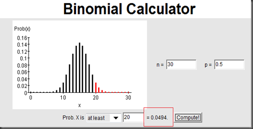
- Under this assumption, we know the the number of winning follows binomial distribution with probability of 0.5. Now we should check Bob’s 20 winning in 30 in this distribution: is this output extreme, or is it a flea?
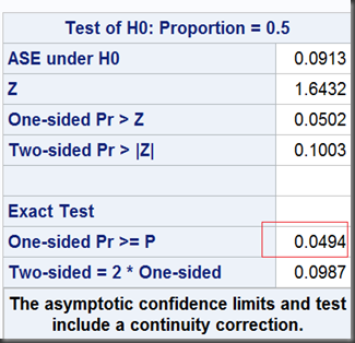
- We then get the p-Value calculated by P(X>=20) which means the chance of winning 20 times and more in 30 games (as extreme or even more extreme ), is 0.0494. Here we only think about winning, so it is a one-sided test. Since this p-Value is less than the default significance level of 0.05 (IT IS A FLEA!), we reject the null and think this is more likely not a fair game (Bob is cheating in this statistical point of view).
That’s all the story. Then this post goes, “Although the procedure is mathematically well defined, it is nonsense”. The following is the first reason listed in the post:
To calculate the probability of Bob’s winning at least 20 games, you use not only the data that you saw (that Bob won 20 games out of 30) but also the imaginary data of Bob winning 21 out of 30 games, or 22 out of 30 games, all the way up to Bob winning all 30 games. The idea of imaginary data is oxymoronic.
In my opinion, the so called “imaginary data” are just the data filling out the binomial distribution (under the assumption of true null hypothesis) we got before and they are not oxymoronic at all (sorry I use “data” as plural).
What do you think? I can’t go far away from here due to my limit knowledge of Bayesian.
————-appendix: SAS Codes and Outputs——————
data a;
input output count;
datalines;
0 20
1 10
;proc freq data=a;
tables output /binomialc (p=0.5) alpha=0.05;
exact binomial;
weight count;
run;

