Statisticians aren’t the problem for data science. The real problem is too many posers — Cathy O’Neil
you actually do need to understand how to invert a matrix at some point in your life if you want to be a data scientist. — Cathy O’Neil
I was asked in several different occasions to explain hypothesis testing to non-technical people in plain English. Now I think I got a pretty neat one while honors belong to three great Germans, Friedrich Engels, Karl Marx, and Heinrich Heine. Engels wrote that Marx once quoted a saying from Heine that “I have sown dragon’s teeth and harvested fleas” (but I didn’t find the original source):
In terms of hypothesis testing, say, if you plant dragon’s teeth, you are not supposed to harvest the fleas; but if you do get the fleas, then most likely they are not dragon’s teeth at all!
To make up the story as simple as possible while keep most of the key messages, here take a one-sample T-test example from SAS TTEST Procedure User Guide, where the investigated data is the Degree of Reading Power (DRP, a measurement of children’s reading skill) from 44 third-grade children. The goal is to test if the mean score of DRP is equal to 30:
Null Hypothesis (H0): μ = 30
Alternative Hypothesis (H1): μ ≠ 30
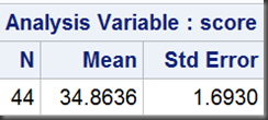
For the following discussion, three statistical measures needed (number of cases, mean and standard error):
proc means data=read maxdec=4 n mean stderr;
var score;
freq count;
run;
and the output:
Here we go:
1. Suppose H0 is true that the mean score is equal to 30 (population mean μ = 30, we assume they are dragon’s teeth!).
2. We know the sample mean is the best estimate of the population mean, here it is 34.8636.
3. This sample mean is derived from a sample (namely, the 44 children). We’d like to know if this sample (with mean of 34.8636) really come from the population (with mean of 30).
4. To get to know this, we can repeat this survey (or trial, experiment), for example, take another 99 samples (also with 44 children in each sample) and calculate their sample means (we then have 100 different means from the whole 100 samples).
5. We may know these means (got from such mechanism), with some necessary mathematical transformation, follow a t-distribution with degree of freedom of 43 (df = 44 – 1):
The denominator as a whole is the standard error.
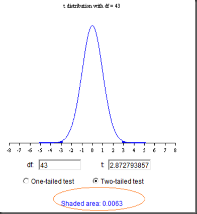
6. Now we can check our interested sample (with mean of 34.8636) in this t-distribution. There is a corresponding t-value of this sample in the distribution, (34.8636 – 30) / 1.6930 = 2.8728:
7. In this distribution, there are only 0.63% (0.0063) of t-values either above 2.8728 or below -2.8728 (symmetry of t-distribution). What does this mean? Obviously, our interested sample (with mean of 34.8636 and t-value of 2.8728) is not in the mainstream of the whole distribution. We can even think it is very “extreme” because, there are only 0.63% of elements in the whole that are more (or at least as equal) extreme than it.
8. We call this number, 0.63% (0.0063) the P-value. According to wikipedia:
the p-value is the probability of obtaining a test statistic at least as extreme as the one that was actually observed, assuming that the null hypothesis is true.
Here the test statistic that was actually observed is 2.8728, the t-value from our interested sample. And we got from this t-distribution that P{|t|>2.8728} = 0.0063.
9. A question is, how extreme is extreme? We can’t define “extreme” exactly, but probably, we can. The threshold is the significance level α (usually 0.05). As a rule of thumb, if p-value is less than the predefine significance level α, then we think the event associated with this p-value is pretty extreme.
10. Retell our story: first we assume the population mean is 30 just as the null hypothesis claims (assume they are dragon’s teeth), and under this assumption, we built a t-distribution; we then got that our interested sample is an extreme case (it is a flea!). It is so extreme (much less than 0.05) that we can even think about that our assumption (the null hypothesis) is far away from true (most likely they are not dragon’s teeth at all!). We reject the null hypothesis and take the alternative that the mean score is different from 30.
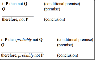
11. Formally, it just follows a simple logic (taken from Glenn Walker and Jack Shostak, P.18):
In our story, P is the null hypothesis, while Q is the extreme case: if H0 is true, most likely such extreme case should not happen; now we observe the extreme case (a t-value of 2.8728 in a t-distribution with degree of freedom of 43), then it is reasonable to question the null hypothesis itself.
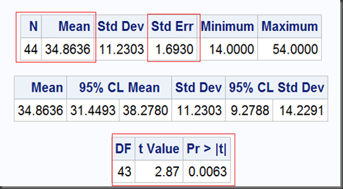
12. To end this analysis, we can take a look at the output of SAS PROC TTEST:
proc ttest data=read h0=30;
var score;
freq count;
run;
The same result (P-value 0.0063 < 0.05, reject H0):
SAS Notes
12. In this example, input data take a form of cell count data, not as raw as the case-record data, so in both PROC MEANS and PROC TTEST, a “FREQ” statement added.
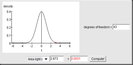
13. You can compute this P-value in step-6 with SAS using ProbT function:
data;
t = 2.8727938571;
df = 43;
tail = 2;
P = tail*(1-probt(t,df));
put P = ;
run;
According to the symmetry of t-distribution, you should multiple 2 to get the two-sided probability:

|
|
14. Long long ago, a so called “critical value” is calculated to support the decision. That’s the calculation method using TINV function:
data;
alpha = 0.05;
tail = 2;
df = 43;tCritic = tinv(1-alpha/tail,df);
put tCritic=;
run;
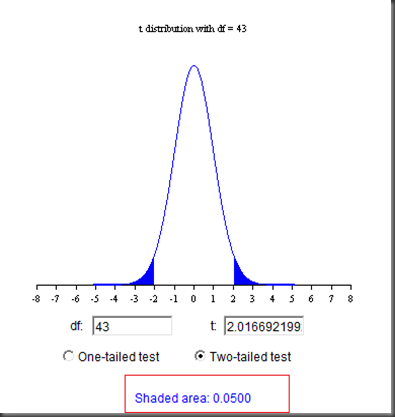
We get this critical value of 2.0166921992:
These two shaded zones are called “rejection zones”. The rule is, if the t-value we observed lies within the rejection zones, we should then reject the null hypothesis and take the alternative. In step-6, the t-value we calculated is 2.8728, which is bigger than this critical value, so we should reject H0.
Critical value approach is equivalent with the p-value approach we discussed before, but slightly old fashioned. P-value is pretty intuitive and can be also easily calculated by computer. In days when computing power was not wildly available, people just took the t-distribution table to look up the critical values.
Most statistical packages including SAS software don’t report the critical value (but still alive in statistics text books).
Reference
Common Statistical Methods for Clinical Research with SAS Examples by Glenn Walker and Jack Shostak
_Hypothesis Testing: A Primer_ (in Chinese)
Two sides T-distribution calculator

