Statistical Notes (5): Confidence Intervals for Difference Between Independent Binomial Proportions Using SAS

A guy notices a bunch of targets scattered over a barn wall, and in the center of each, in the “bulls-eye,” is a bullet hole. “Wow,” he says to the farmer, “that’s pretty good shooting. How’d you do it?” “Oh,” says the farmer, “it was easy. I painted the targets after I shot the holes.” – An Old Joke

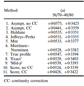
Note on how to get the difference between independent binomial proportions using SAS PROC FREQ (tested in SAS 9.3M1).  Also, benchmarks took from Prof. Newcombe ’s paper:

Interval estimation for the difference between independent proportions: comparison of eleven methods.

Key findings (SAS output):

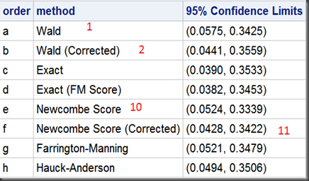
1. SAS Proc Freq offers 8 ( including 4 of total 11 in Prof. Newcombe ’s paper) methods to compute confidence intervals for difference between independent binomial proportions:

• Wald #1
• Wald (Corrected) #2
• Exact
• Exact (FM Score)
• Newcombe Score #10
• Newcombe Score (Corrected) #11
• Farrington-Manning
• Hauck-Anderson

Note that #1 method is the most popular one in textbook, #10 might  be the most wildly used method in industry.

2. There is a big discrepancy in the outputs in the  so called “exact” method among  SAS Proc Freq and Prof. Newcombe ’s paper. Seems they used different methods (in the same “exact” families) under same name. Needs further investigation.

The SAS codes:

/*
2*2 table

        response0 response1
group1      56      14
group2      48      32
*/

data ci;
    input grp res count;
datalines;
1 0 56
1 1 14
2 0 48
2 1 32
;

/*
methods:
Exact
Farrington-Manning
Hauck-Anderson
Newcombe Score
Wald
*/
ods select  PdiffCLs;
ods output PdiffCLs=ci1;
proc freq data=ci order=data;
    tables grp*res /riskdiff (CL=(EXACT FM HA WILSON WALD));
    weight count;
    exact riskdiff;
run;

/*
methods:
Exact (FM Score)
*/
ods select  PdiffCLs;
ods output PdiffCLs=ci2;
proc freq data=ci order=data;
    tables grp*res /riskdiff (CL=(EXACT));
    weight count;
    exact riskdiff(fmscore);
run;

/*
methods:
Newcombe Score (Corrected)
Wald (Corrected)
*/
ods select  PdiffCLs;
ods output PdiffCLs=ci3;
proc freq data=ci order=data;
    tables grp*res /riskdiff (CORRECT CL=(WILSON WALD));
    weight count;
    exact riskdiff;
run;

/put them all/
data CI_all;
    set ci3 ci2 ci1;
    CI=‘(‘||compress(put(LowerCL,8.4))||’, ‘||compress(put(UpperCL,8.4))||’)’;
run;

proc sql;
    select
    case Type
        when “Wald” then “a”
        when “Wald (Corrected)” then “b”
        when “Exact” then “c”
        when “Exact (FM Score)” then “d”
        when “Newcombe Score” then “e”
        when “Newcombe Score (Corrected)” then “f”
        when “Farrington-Manning” then “g”
        when “Hauck-Anderson” then “h”
        else “i”
    end as order,
        Type “method”,
        CI “95% Confidence Limits”
    from CI_all
    order by order
        ;
quit;

———————————-

You may be also interested in this post on calculating confidence intervals for single proportion:

Statistical Notes (3): Confidence Intervals for Binomial Proportion Using SAS

using the following 11 methods:

• 1.  Simple asymptotic, Without CC | Wald
• 2.  Simple asymptotic, With CC      
• 3.  Score method, Without CC | Wilson       
• 4.  Score method, With CC    
• 5. Binomial-based, ‘Exact’ | Clopper-Pearson              
• 6.  Binomial-based, Mid-p      
• 7.  Likelihood-based            
• 8.  Jeffreys    
• 9.  Agresti-Coull,z^²⁄₂ successes          
• 10. Agresti-Coull,2 successes and 2 fail           
• 11. Logit